Oral Abstracts Session

Halil Noyan, MD
Medical Student
Charité – Universitätsmedizin Berlin
Berlin, Berlin, Germany
Halil Noyan, MD
Medical Student
Charité – Universitätsmedizin Berlin
Berlin, Berlin, Germany

Richard Hickstein, MD
Physician and Researcher
Charité – Universitätsmedizin Berlin
Berlin, Berlin, Germany
Christian Lim
Clinical Researcher
Working Group on CMR, Experimental and Clinical Research Center, a cooperation between Charité – Universitätsmedizin Berlin and the Max Delbrück Center for Molecular Medicine in the Helmholtz Association, Berlin, Germany, Germany

Clemens Ammann, MD
Physician
Charité – Universitätsmedizin Berlin
Berlin, Berlin, Germany

Thomas C. R Hadler, PhD
Postgraduate
Charité - Universitätsmedizin Berlin
Berlin, Berlin, Germany
Christian Hickstein
Researcher
Technische Universität Berlin, Faculty IV – Electrical Engineering and Computer Science, Institute of Software Engineering and Theoretical Computer Science, Straße des 17. Juni 135, 10623 Berlin, Germany, Germany
Johanna Kuhnt
Medical student
Charité – Universitätsmedizin Berlin, Germany
Elias Daud, MD
Physician
Charité – Universitätsmedizin Berlin, Germany

Edyta Blaszczyk, MD
Cardiologist
Charité - Universitätsmedizin Berlin
Berlin, Berlin, Germany

Jeanette Schulz-Menger, MD
Head Working Group Cardiac MRI
Charité/ University Medicine Berlin and Helios
Berlin, Berlin, Germany
Comparison | Dice [-] (95% CI) | HD95 [mm](95% CI) | RVD [%] (95% CI) | ΔVol [ml] (95% CI) |
nnU-Net modelvs. O1 | 0.80 ± 0.03(0.78–0.81) | 2.01 ± 1.84(1.77–2.25) | 8.55 ± 10.40(2.27–14.49) | 5.81 ± 6.86(1.76–9.77) |
O1 vs. O2 | 0.69 ± 0.12(0.62–0.76) | 3.96 ± 2.35(2.65–5.41) | 23.58 ± 20.86(12.92–37.03) | 14.12 ± 7.93(9.59–18.86) |
Intraobserver (O1) | 0.82 ± 0.06(0.79–0.86) | 1.70 ± 0.72(1.24–2.07) | 0.94 ± 8.63 (-3.75–6.32) | -0.40 ± 4.77(-3.17–2.39) |
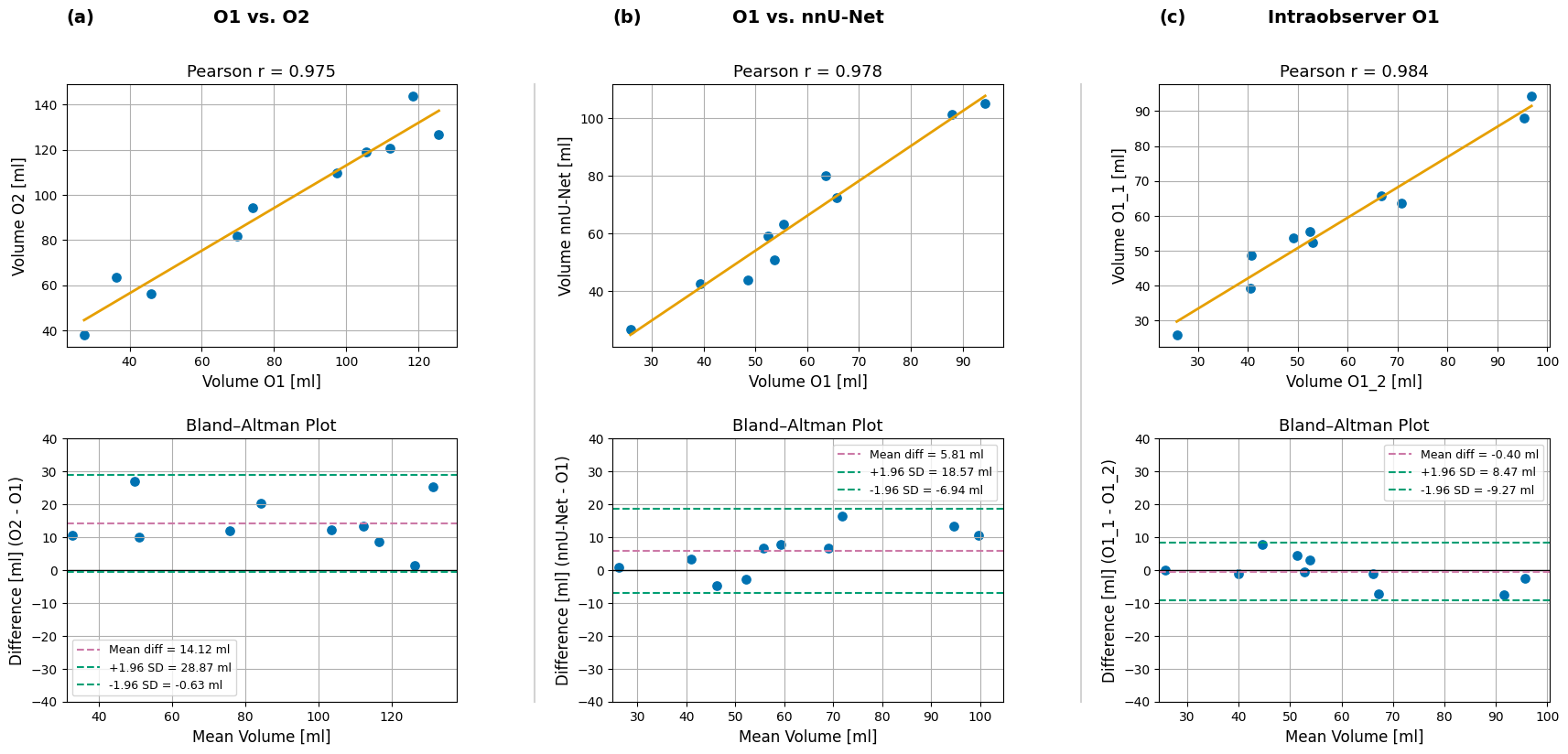
.png) Figure 2: (a) Interobserver comparison between two readers (O1 vs. O2), (b) comparison between the nnU-Net model and reader O1, and (c) intraobserver comparison for reader O1. The top row shows Pearson correlation plots, and the bottom row shows the corresponding Bland–Altman plots. The limits of agreement in the Bland–Altman plots were defined as the mean difference ± 1.96 × the standard deviation of the differences.
Figure 2: (a) Interobserver comparison between two readers (O1 vs. O2), (b) comparison between the nnU-Net model and reader O1, and (c) intraobserver comparison for reader O1. The top row shows Pearson correlation plots, and the bottom row shows the corresponding Bland–Altman plots. The limits of agreement in the Bland–Altman plots were defined as the mean difference ± 1.96 × the standard deviation of the differences.